In my first post, I described the general logic of Bayes factors. I will continue discussing the general logic of Bayes factor, while introducing some of the basic functionality of the BayesFactor package.
Recap: What is a Bayes factor?
The Bayes factor is the relative evidence provided by the data for comparing two statistical models. It has two equivalent definitions:- The Bayes factor is the relative predictive success between two hypotheses: it is the ratio of the probabilities of the observed data under each of the hypotheses. If the probability of the observed data is higher under one hypothesis than another, then that hypothesis is preferred.
- The Bayes factor is evidence: it is the factor by which the relative beliefs must be multiplied after the data have been observed, providing new (posterior) relative beliefs. The stronger the evidence, the more beliefs must change.
Student's sleep data
Student (1908) describes a study by Cushny and Peebles (1905) on the effect of several medications on sleep. One of the drugs they studied was Laevo-hyoscine hydrobromide, which we'll abbreviate as “LH”. LH was administered to 10 patients on several nights, and the average amount of sleep over the patients' unmedicated sleep (measured on other nights) was recorded. For the purposes of this post, we will make the typical assumptions about the data that would be made if we were to apply the \(t\) procedure: specifically, that the observation are independent and normally distributed.We return to Carole and Paul, who have another disagreement. Carole does not believe that LH increases sleep at all, while Paul claims that it does. This would traditionally be handled by a t test. Under Carole's hypothesis, the \(t\) statistic has a Student's \(t\) distribution with \(N-1\) degrees of freedom. That is, \[ t = \frac{\bar{y}}{s}\sqrt{N} \sim \mbox{Student’s }~t_{N-1} \]
Another way of stating her prediction is in terms of the observed effect size, \(\hat{\delta}=\bar{y}/s\), which is shown in the figure below. It is simply a Student's \(t\) distribution, scaled by \(1/\sqrt{N}\).

Paul's hypothesis — that LH causes an increase in sleep — is problematic. Typically, we require scientific hypotheses to constrain the data in some way. We require them to predict that some outcomes are more plausible than others. Paul's hypothesis, however, predicts nothing. His hypothesis does not constrain the data.
This highlights a curious fact about traditional significance testing. The only hypothesis we can support using a classical significance test is the one that makes no predictions! If we applied the traditional t test to these data, we could only reject Carole's hypothesis in favor of Paul's — but never support Carole's — even though Paul has advanced a decidedly unfalsifiable hypothesis.
To be testable, Paul's hypothesis must make predictions, as Carole's has. As a first step, let's assume that Paul believes that LH will increase sleep by 1 standardized effect size unit. If \(\mu\) is the mean increase in hours of sleep and \(\sigma\) is the standard deviation of the increases, then the standardized increase is \[ \delta = \frac{\mu}{\sigma}. \] and Paul believes that \(\delta=1\). Using the noncentral t distribution, we can obtain Paul's predictions for the observed effect size \(\hat{\delta}\), shown in the figure below:

As expected, the predictions are centered around \(\hat{\delta}=1\). We now have two hypothesis: Carole believes that \(\delta=0\), and Paul believes that \(\delta=1\). These hypotheses imply two different predictions for the observed effect size, as shown above. We can now compare the predictions with the results presented by Student to see whether Paul or Carole is favored by the evidence.
The
sleep data set is built into R; the following R code will extract the data for LH (which is labelled group 2):improvements = with(sleep, extra[group == 2]) improvements
## [1] 1.9 0.8 1.1 0.1 -0.1 4.4 5.5 1.6 4.6 3.4

We begin our analysis by computing \(N\) and the \(t\) statistic from the data:
N = length(improvements)
t = mean(improvements)/sd(improvements) * sqrt(N)
t
## [1] 3.68
deltaHat = t/sqrt(N)
deltaHat
## [1] 1.164
The figure below shows both Carole's and Paul's predictions for the observed effect size as overlapping gray distributions. The observed effect size is denoted by the vertical line segment. In order to compute the Bayes factor, we must compare the relative heights of the two distributions for the observed data. The probability density of the observed data is 67.9451 times higher under Paul's hypothesis than under Carole's. The Bayes factor favoring Paul is thus 67.9451.

We can easily compute this using R's built in functions. Under Carole's hypothesis, the \(t\) statistic has a central \(t\) distribution with 9 degrees of freedom; Under Paul's hypothesis, the \(t\) statistic has a noncentral \(t\) distribution with 9 degrees of freedom, and a noncentrality parameter of \(\delta\sqrt{N}=1\times\sqrt{10}\). The ratio of the two densities, at the observed \(t\) statistic, yields the Bayes factor.
dt(t, df = 9, ncp = 1 * sqrt(10))/dt(t, df = 9)
## [1] 67.95
Uncertain hypotheses, and a first look at BayesFactor
In the section above Carole's and Paul's original hypotheses, when stated in terms of effect sizes, were \[ \begin{align*} {\cal H}_c : \delta &= 0\\ {\cal H}_p : \delta &> 0; \end{align*} \] that is, Paul hypothesized that the drug increases sleep on average, and Carole hypothesized that it had no effect. The problem with this was that Paul's hypothesis was untestable, because it does not lead to any proper constraint on the data.The solution is for Paul to propose a hypothesis that does constrain data. We chose the hypothesis \(\delta=1\) for Paul, and showed how that can be used to compute a Bayes factor. The resulting Bayes factor, however, does not seem to capture very well the spirit of Paul's original hypothesis. Paul was not specific about what the exact effect size was. But \(\delta>0\) won't do either; it is so unspecific as to be completely unfalsifiable.
What we need is a middle ground between the two. In the previous post I showed how a Bayesian analysis can spread uncertainty out over a range of parameter values using a probability distribution.
The figure below shows two hypotheses: Carole's null hypothesis (\(\delta=0\)) whose predictions I've already presented, and a plausible hypothesis for Paul (\(\delta>0\)). Under Paul's hypothesis, plausible effect sizes are not spread evenly across the positive effect sizes, because that would not lead to any constraint on the data. Instead, small effect sizes are preferred to large ones. It is implausible for the effect size to be too large, so the plausibility of the effects diminish as the effect sizes get larger.
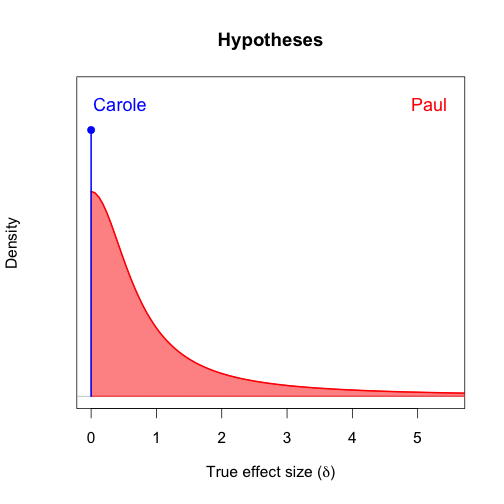
The shape of this prior distribution is the positive half of a Cauchy distribution, or a Student's \(t\) distribution with 1 degree of freedom. The Cauchy prior was suggested by Rouder et al. (2009), and is the one implemented in the
BayesFactor package.Of course, this half-Cauchy distribution is not the only way we could implement Paul's hypothesis. We could choose a different shape of distribution; we could make it wider or narrower around 0; we could even restrict the range further. We must choose some valid probability distribution in order to create a hypothesis that constrains the data, and we should do our best to make the test meaningful by choosing a defensible distribution.
Recall from the previous post that the way we obtain predictions from an uncertain hypothesis like Paul's, we weight the predictions for each possible \(\delta\) by their plausibility and average them. This is represented by the integral: \[ P(\hat{\delta}\mid{\cal H}_p) = \int P(\hat{\delta}\mid \delta)p(\delta)\,d\delta, \] where \(P(\hat{\delta}\mid \delta)\) gives the predictions for a specific \(\delta\), and \(p(\delta)\) is the distribution in the figure above, giving the weightings for all possible values of \(\delta\).
The figure below shows Carole's predictions (which are the same as before) and Paul's new predictions for the observed effect size. Notice that Paul's predictions are now substantially more spread out than before. The uncertainty Paul has about the true value of \(\delta\), added to the uncertainty that is inherent in the sampling given a particular true value, has caused his predictions to be less certain. This spreading out is the penalty for a having a less-specific hypothesis.

Now that we have predictions from both Carole's and Paul's hypothesis, we can compute a Bayes factor. The Bayes factor is the ratio of the heights at the observed \(\hat{\delta}\) value, shown in the figure below by the vertical line segment. The Bayes factor is 21.3275 in favor of Paul, because the probability density of the observed data is 21.3275 times greater under Paul's hypothesis than under Carole's. Note that this is substantially lower than the Bayes factor in favor of Paul's hypothesis when it was more specific. More flexible hypotheses, like Paul's, are automatically penalized by the Bayes factor.

As previously mentioned, the distribution used as Paul's hypothesis happens to be the one implemented in the
BayesFactor package. We can thus use the function ttestBF, part of the package's suite of functions, to compute the Bayes factor for the Student sleep data.If you have not installed the
BayesFactor package yet, install the package first (help here). If you define the improvements vector as above, you can run the following two lines of code to load the package and perform the a Bayes factor \(t\) test. The nullInterval argument tells ttestBF that you want to consider that range as a hypothesis. Paul's hypothesis ranged from 0 to \(\infty\), so we specify that range using the nullInterval argument:library(BayesFactor) ttestBF(improvements, nullInterval = c(0, Inf))
## Bayes factor analysis
## --------------
## [1] Alt., r=0.707 0<d<Inf    : 21.33  ±0.01%
## [2] Alt., r=0.707 !(0<d<Inf) : 0.1036 ±1.4%
##
## Against denominator:
##   Null, mu = 0
## ---
## Bayes factor type: BFoneSample, JZS
[1] and [2] The first line is the one we specified, where \(0<d<\infty\). The second Bayes factor is the Bayes factor for the complement of the specified range (the ! indicates negation) — in this case, the negative effect sizes. Each of the two lines contains three pieces of information: the numerator hypothesis for the Bayes factor, the Bayes factor itself, and a measure of the error in the estimate of the Bayes factor. Here, the error is very small.Below the two Bayes factors, the denominator hypothesis is specified. The denominator is the hypothesis to which all the numerator hypotheses have been compared. The first Bayes factor, then, is the comparison of the positive effect sizes to the null hypothesis; the second Bayes factor is the comparison of the negative effect sizes to the null. The positive hypothesis is preferred to the null hypothesis, and the null hypothesis is preferred to the negative hypothesis.
In order to gain some insight into the Bayes factor, one can compute the Bayes factor for a range of possible data. The figure below shows the Bayes factors for a range of observations. The effect size in the Student sleep data is denoted by the circle. Observing smaller effect sizes or negative effect sizes favors Carole's hypothesis (the null), while observing larger effect sizes favors Paul's alternative.

Conclusions
What can we conclude from our Bayes factor analysis? Paul's alternative hypothesis was favored to Carole's null hypothesis by a factor of 21.3275, suggesting a substantial amount of evidence in favor of a positive effect size. This is, of course, conditioned on the “reasonableness” of Paul's hypothesis. The Bayes factor is not, however, arbitrary: although the Bayes factor would change if we changed the prior, we would have to choose a strange prior to change the substantive conclusion.In the next post, we will explore the
BayesFactor package's \(t\) tests in more detail.
Hi,
ReplyDeleteReally helpful post - thanks for writing it (and the BF package too!) I was hoping you may be able to help with one area that I can't quite figure out:
With Paul's second prior, the half-cauchy, the prior likelihood on negative effect sizes is 0. The integral involves a multiplication with this prior, so every negative effect size should have probability zero (according to my understanding), yet in the third from last figure the distribution over negative values has positive likelihoods.
Intuitively it makes sense that if the real effect size is close to 0 but positive, that you would still expect to observe negative effect sizes an a small portion of trials by chance, but I can't figure out the math behind going from the half Cauchy to this distribution which has non-zero likelihood for negative values of delta hat.
Is the math/code behind this transition relatively trivial as it was in the previous example and if so, would you be willing to share it?
Any help would be greatly appreciated! Thanks,
Ben
Good information and, keep sharing like this.
ReplyDeleteCrm Software Development Company in Chennai
Best Corporate Video Production Company in Bangalore and top Explainer Video Company in Bangalore , 3d, 2d Animation Video Makers in Chennai
ReplyDeleteGreat article. Thanks for it.